
A Geometric Interpretation of Correlations
Correlations have a surprising geometric interpretation that demystifies some of their properties

Have you ever wondered why correlations share so many similarities with cosines? Both are bounded by -1 and +1 and both have inequalities similar to ones you'd expect for dot products of unit vectors. For example, if we know X and Y are perfectly correlated (=+1), and Y and Z are perfectly anti-correlated (=-1) it must follow that X and Z are perfectly anti-correlated (=-1). This is more than just a coincidence.
The following is an attempt to give a geometric point of view on correlations that might change how you think about them. I hope you enjoy.
First, some needed background.
Correlations, Covariance, and All that
Let's now define the correlation between two random variables X and Y as:
Where
and,
Enter the Matrix
Now imagine instead of only two variables we had several of them. Let X = (X₁, X₂, ..., Xₙ) be a random vector, where Xᵢ for any i is a random variable.
We can define a covariance matrix as follows:
In matrix notation this becomes:
Note: Cov(X,Y) is something else called the cross-variance matrix.
What's important for us is that they have two special properties:
They're positive definite e.g. aᵀCₓₓa ≥ 0
And Cₓₓ is symmetric, i.e. Cₓₓᵀ = Cₓₓ
The first property (positive definiteness) can be understood as the variance of a linear recombination of the components of X. Variance is always non-negative. The second property shouldn't be surprising as the correlation of i with j should be equal to the correlation of j and i.
We can define the correlation matrix of n random variables X₁,...,Xₙ is the n × n matrix C whose (i,j) entry is
In matrix notation this can be written as:
Where X̃ = (X₁/σ(X₁), X₂/σ(X₂), ..., Xₙ/σ(Xₙ))
The correlation matrix is manifestly invariant with respect to affine transformations (any scale and shift) of the vector X as the mean is explicitly subtracted out of each element and the denominator of each element is explicitly divided.
So in other words:
Where X̂ is a unit vector with zero mean. Henceforth we will drop the ^ and element-wise this is.
Consider that as Xᵢ is actually a random variable to compute this we either need to gather a data sample to approximate it or without data we must consider Xᵢ(ω) as a function of elements ω in the probability space Ω in other words:
This is actually an infinite dimensional dot product (over a Hilbert "space" if that's your thing). This kind of leaves us in a bind and far from our goal of representing this as a vector dot product, but it turns out we can simulate this to arbitrary precision as the dot product of two vectors that will give us the same result.
There are two ways to do this:
To grab m data points sampled from the distribution
Skip that and actually decompose a concrete correlation matrix via the Cholesky decomposition
Introducing Cholesky Decompositions
It turns out every symmetric and positive definite matrix (like correlation matrices) can be decomposed into the product of a lower triangular matrix and its transpose.
So C = LLᵀ
Here, L is a real lower triangular matrix with positive diagonal entries.
If we have a vector ε with each element sampled independently from the standard normal distribution, by definition the covariance matrix will be the unit matrix on average.
However, if we multiply by L, Lε will have correlation C.
Since we're interested in these triangle inequalities, let's work with three random variables.
Consider three random variables X, Y, Z. We can write down their correlation matrix:
And break them down according to Cholesky.
Note that:
This is manifestly symmetric and with some work can be shown to be positive definite.
Applying L to our noise vector yields:
Because the different εᵢ are orthogonal in expectation we can express X, Y, Z as vectors.
Taking the various dot products we can confirm:
We can also confirm that they are indeed unit norms because we can just read off C as a function of the ℓs:
And that therefore they are cosines and not just dot products!
Now for the other side of the proof, we can compute the correlation matrix.
Since ε₁,ε₂,ε₃ are independent standard normals, we have:
E[εᵢ]=0, E[εᵢ²]=1, and E[εᵢεⱼ]=0 for i≠j
Let's compute Cov(X,Y)=E[(X-E[X])(Y-E[Y])]. Since E[X]=E[Y]=0:
Cov(X,Y)=E[XY]
Substitute X and Y:
Distribute:
Because ε₁ and ε₂ are independent and have zero mean:
E[ε₁ε₂]=0 and E[ε₁²]=1
Thus:
Similarly, we can compute:
By the same logic:
And for Corr(Y,Z):
Expanding and using the independence and zero-mean conditions:
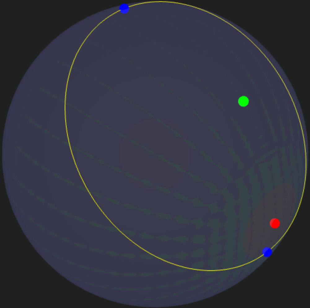
To summarize, we proved that correlations can be viewed as dot products on a unit sphere, which naturally introduces an angle related to each and every correlation.
So from now one when you think of correlations you hopefully are imagining unit vectors on a sphere.
Now for bonus points, now that we know these correlations are secretly dot products of unit vectors on the sphere lets us use the usual triangle inequalities on metrics to construct closely related inequalities on the correlations themselves.
Triangle inequality demystified
We can now define a distance between two variables X, Y based on their correlation c_{xy}
which obeys the metric properties
θ(X,Y) ≥ 0
θ(X,Y) = θ(Y,X)
θ(X,X) = 0
θ(X,Y) ≠ 0 if X ≠ Y
Given that it's a metric we get the triangle inequality for free:
So in other words: θ(X,Z) ≤ θ(X,Y) + θ(Y,Z)
We can also see that θₘᵢₙ(X,Z) = |θ(X,Y) - θ(Y,Z)| and of course θₘₐₓ(X,Z) = θ(X,Y) + θ(Y,Z)
Given that, we can infer the min correlation max(c_{xz}) = cos(|θ(X,Y) - θ(Y,Z)|) and min(c_{xz}) = cos(θ(X,Y) + θ(Y,Z))
Writing this as a function of the original correlations (with some trig-jujitsu which I'll spare you):